Dissecting Softmax
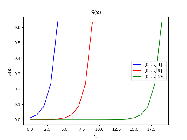
The best way to understand the behavior of any function is to plot it. But softmax is no ordinary function. It takes a vector and maps it to another vector. In more technical terms, softmax can be regarded as a multivariate and vector-valued function. There is no general method for visualizing such a function in 2-D, or even 3-D, spaces, as we typically do for functions over scalars. Yet, for a given input vector, we can plot the output of softmax over that input. There is a caveat though. If the input vector contains repeated elements, the resulting plot may not convey the complete picture. Additionally, when plotting softmax in this manner, we essentially disregard the order of the elements. Plotting the softmax of [1, 2] will be the same as that for [2, 1]. Nevertheless, this is the best way we have for visualizing softmax, and I will frequently use it in this post. The following diagram shows softmax applied to 3 integer vectors [0, …, 4], [0, …, 9], and [0, …, 19].
Softmax is one of the most important and popular activation functions used in machine learning. Activation functions serve a crucial role in artificial neural networks. Their primary purpose is to introduce non-linearities into the network, enabling it to learn complex patterns and relationships in the data. Intuitively, softmax maps a vector of real numbers to a probability distribution. That is why softmax is often used as the last layer activation function in many neural networks, including LLMs.
Suppose that you have the following vector:
| -1 | 0.5 | 5 | -0.3 | 1 | 1.7 | 0.6 | 3.2 |
This could be a datapoint you found somewhere, or the output from a dense layer in a neural network. When applying softmax to this vector, you get a vector of the same size, but each of the values in the new vector will be between 0 and 1, and their sum will be 1:
| 0.00198 | 0.00888 | 0.79913 | 0.00399 | 0.01464 | 0.02947 | 0.00981 | 0.1321 |
| Sum: | 1.0 | ||||||
Apart from 0.79913, which corresponds to the largest value in the input vector, all other values are very small.
Mathematical formulation of softmax
To get deeper into understanding softmax, let’s take a look at its mathematical formulation. As we just saw, softmax transforms a vector of real numbers to another vector of the same size. The values of the output vector are all in the [0, 1] range, or more accurately the (0, 1] range, as we will see. Mathematically, we write:
\[S_k: \mathbb{R}^k \rightarrow (0,1]^k\]where $S_k$ denotes the softmax function over the domain $\mathbb{R}^k$, $\mathbb{R}$ denotes the set of real numbers, and $k$ denotes the length of the input, and output vectors. For simplicity, in the following, we often drop the $k$ subscript from $S_k$ , and use $S$ to refer to the softmax function.
For an input vector $\mathbf{x}$, each element of $S(\mathbf{x})$ is calculated using the following formula:
\[S(\mathbf{x})_i = \frac{e^{x_i}}{\Sigma_{j=1}^k{e^{x_j}}}\]In other words, we compute the $i$th element of the output vector by dividing the exponential of the $i$th element of the input (i.e., Euler’s number $e$ raised to the power of $x_i$) by the sum of exponentials of all elements in the input vector. As pointed out in the original softmax paper, softmax is a Normalized Exponential transformation.
From the formula, we can see that each element of $S(\mathbf{x})$ is in fact in the range (0, 1]. Additionally, we can see that the sum of all elements of $S(\mathbf{x})$ is 1. This is why the output of softmax is interpreted as a probability distribution. This behavior makes softmax suitable for multiclass classification problems, where each class has a probability associated with it.
A special case is when all $x_i$’s in the input vector $\mathbf{x}$ are the same. In this case, all $S(\mathbf{x})_i$’s will be the same as well, and since they add up to 1, they will all be equal to $\frac{1}{k}$, where $k$ is the length of vector $\mathbf{x}$. In this case, the output vector $S(\mathbf{x})$ represents a discrete uniform probability distribution.
Softmax magnifies differences
It is often said that softmax is sensitive to differences in input values, and magnifies those differences. In this section, I want to understand what that actually means.
If I apply softmax to $\mathbf{x} = [-10.0, -9.5, -9.0, …, 0, …, 9.5, 10.0]$, the resulting vector will contain very small values in the range [8.11e-10, 0.39]. What is magnifying about that?
Let’s see if visualization can help. For the vector $\mathbf{x}$ above, the following diagram shows $S(\mathbf{x})$ plotted over $\mathbf{x}$.
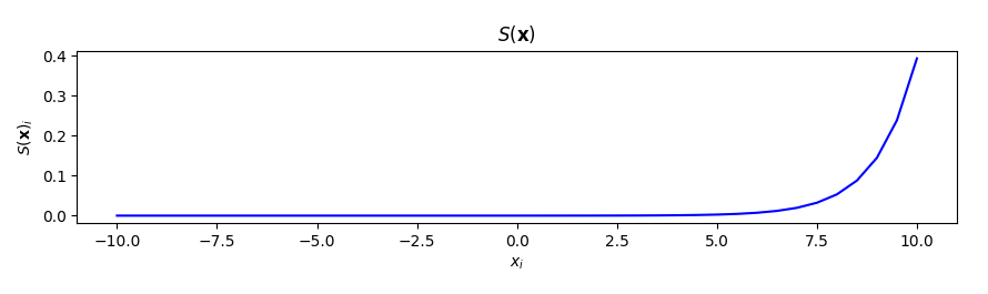
The graph resembles an exponential curve. We can express this curve using a function $f(.)$ such that $f(x_i) = S(\mathbf{x})_i$. Using the formula of softmax, we can see that $f(x_i) = \frac{e^{x_i}}{A}$, where $A$ is the sum of exponentials of elements of vector $\mathbf{x}$ above, and is equal to $55980.13$. Note that $f(.)$ is different from $S(.)$. The latter takes a vector as input, while the former takes a scalar as input and is a function that we can easily plot. The curve shown in the diagram above is an excerpt of the graph of $f(.)$ in the [-10, 10] range. The slope of this curve changes as we move along the x-axis. In fact, since $A$ is constant, it is easy to see that the derivative of $f(.)$ (which gives the slope of the curve at each point) is equal to $f(.)$ itself! We have $f’(.) =f(.)$. Note that we are not computing the derivative of softmax, just that of the curve shown in the diagram. At $x_i=-10$ the value and slope of the function are both $8.11e-10$ (almost zero), whereas at $x_i=10$ they are both $0.39$ (note that the x:y aspect ratio of the diagram is 1:10, so the curve looks a lot steeper than $0.39$)!
So even though values on the y-axis are all very small, they grow exponentially with changes in $x_i$. We can see this mathematically by looking at the ratios of elements of $S(\mathbf{x})$:
\[\forall i, j: \frac{S(\mathbf{x})_i}{S(\mathbf{x})_j} = e^{x_i-x_j}\]Each unit of change in the input vector, results in a change by a factor of $e$ in the output vector. This is what they refer to as the magnifying effect of softmax on differences in the input vector.
As mentioned above, softmax is sensitive to differences in the input vector. So if we increase or decrease all elements of the input vector a by a scalar, thereby maintaining the relative differences, the softmax of the resulting vector should be the same as the softmax of the original vector. In other words:
\[S(\mathbf{x} + c) = S(\mathbf{x})\]We can show that this is true by applying the formula of softmax, and using the fact that $e^{x_i+c}=e^{x_i} \times e^c$.
In practice, $S(\mathbf{x}+c) = S(\mathbf{x})$ plays an important role in stabilizing softmax implementations. Many softmax implementations internally compute $S(\mathbf{x}-max(\mathbf{x}))$ (see example), as opposed to $S(\mathbf{x})$, to avoid numerical overflow or underflow that may happen when computing exponentials, if $\mathbf{x}$ contains very large positive, or very small negative values.
Scaling the input vector
How about multiplying each element of the input vector by a constant $c$?
It is not so straightforward to specify $S(c\mathbf{x})$ in terms of $S(\mathbf{x})$, but we can compare the magnifying effect of softmax on $\mathbf{x}$ and $c\mathbf{x}$. Let $\mathbf{s} = S(\mathbf{x})$ and $\mathbf{w} = S(c\mathbf{x})$. In this case we have:
\[\frac{w_i}{w_j} = e^{cx_i-cx_j} = e ^{c(x_i-x_j)} =(e^{x_i-x_j})^c = (\frac{s_i}{s_j})^c\]To express this in words, multiplying elements of the input vector by a constant results in an exponential growth in the magnifying effect of softmax on differences. Note that $c$ can be larger or smaller than 1. In the former case ($c>1$), smaller values in the input will be squashed more quickly. We see that in the following diagram, which shows $S(c\mathbf{x})$ plotted over $\mathbf{x}$, for $\mathbf{x}=[1, 2, 3, 4, 5, 6]$. As we go from left to right, we double the value of $c$ in each step, from 1 up to 8.
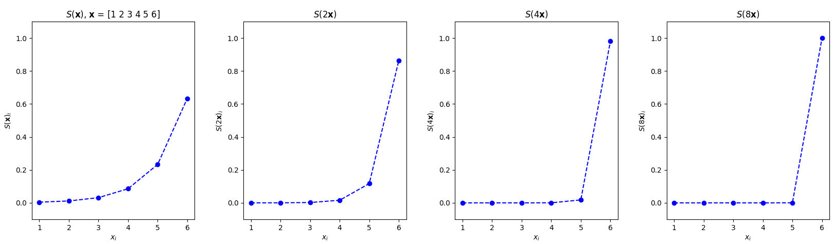
As we increase $c$, the tail (corresponding to smaller values in $\mathbf{x}$) is squashed and flattened more dramatically. Here, each unit of change in vector $\mathbf{x}$ results in a change by a factor of $e^c$ in the output vector.
The last diagram is particularly of interest. The output of softmax in this case is the vector $[1.6e-28, 1.4e-21, 1.3e-14, 1.1e-07, 9.99999887e-01]$, which is approximately equal to $[0, 0, 0, 0, 0, 1]$. In fact, if we increase $c$ even further, in the limit, $S(c.\mathbf{x})$ will be $[0, 0, 0, 0, 0, 1]$. This vector is the one-hot representation of $5$, the index of the largest element of $\mathbf{x}$ (and $c.\mathbf{x}$), or the argmax of $\mathbf{x}$ (and $c.\mathbf{x}$).
Mathematically speaking, argmax of a function $f(.)$ over a subset $Z$ of its domain is a member $z \in Z$ for which $f(z)$ has the maximum value of $f(.)$ over $Z$:
\[argmax_Z(f) = \{ z \in Z | \forall x \in Z: f(x) \leq f(z) \}\]In machine learning literature and use cases, argmax is often applied to a vector (as opposed to a function), and returns the index of the largest element in the vector. As hinted above, this index can be represented as a one-hot vector.
Going back to our example above, we see that with a sufficiently large $c$ and a bit of approximation, softmax behaves like argmax with one-hot representation. In fact, a more accurate name for softmax that is used in some literature is softargmax.
In the diagram above, we could also go in the opposite direction and reduce $c$. By reducing $c$, or multiplying the input vector by a factor smaller than 1 ($c<1$), we can turn argmax into a top-k selector.
Does that ring a bell?
Suppose that you have a neural network, with softmax as its last layer activation function, and have trained the model on a classification task to predict the best matching class for any given input. Ideally, you have trained the model such that the output of the softmax activation function, when plotted over its input (vector $\mathbf{z}$ in the following diagram), resembles the rightmost plot in the diagram above (i.e., the plot with the lowest entropy).
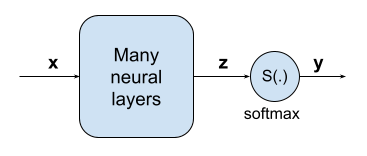
At the inference time, you can simply use this for top-k sampling by multiplying the input to softmax (vector $\mathbf{z}$ above) by a parameter $c<1$, to make softmax behave more like the leftmost plot (with the highest entropy), in the previous diagram. In LLMs, a similar mechanism is used via the temperature parameter to control the diversity of the generated output.
Does softmax have a fixed point?
As mentioned earlier, softmax is a normalization function, and its output can be interpreted as a discrete probability distribution. Most normalization functions, such as z-score normalization and min-max normalization, when applied to data that is already normalized using the same method, do not produce new results. In other words, for these normalization functions, $N(N(\mathbf{x})) = N(\mathbf{x})$. Does the same property hold for softmax? In other words, if we apply softmax to a vector that already is a probability distribution will the result be the same as the input probability distribution? To answer this question, in this section we are going to compute the fixed point of softmax. In other words, we want to find vectors for which the following equation holds:
\[S(\mathbf{x}) = \mathbf{x}\]We know that $\mathbf{x}$ is a vector. For $S(\mathbf{x}) = \mathbf{x}$ to hold, all elements of $S(\mathbf{x})$ must be equal to their corresponding elements in $\mathbf{x}$. In other words, for each element $x_i$ of $\mathbf{x}$, the following equation must hold:
\[x_i = S(\mathbf{x})_i = \frac{e^{x_i}}{\Sigma_{j=1}^k{e^{x_j}}}\]We can rewrite this as follows:
\[x_i \Sigma_{j=1}^k{e^{x_j}} = e^{x_i}\]This equation is not very easy to solve. So let’s start with building some intuition with a simple example. For this, I decided to repeatedly apply softmax to its output, with [0, 1] as the starting input vector. In each iteration, the result of applying softmax is a 1-D vector of length 2, just like [0, 1] is. If we plot these vectors as points in the cartesian plane, we get the following diagram.
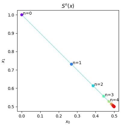
Each point in the diagram represents $S^n([0, 1])$, where $S^n(.)$ denotes the composition of softmax with itself $n$ times. We also define $S^0(\mathbf{x})$ to be $\mathbf{x}$.
As we can see in the diagram, repeatedly applying softmax, starting from $[0, 1]$ brings the output closer and closer to $[0.5, 0.5]$. In fact, $[0.5, 0.5]$ is the fixed point of softmax for 1-D arrays of length 2. There is nothing special about $[0, 1]$, and if we’d started from any other vector ($[0.5, 1]$ is a fun one), and repeatedly applied softmax, again we’d end up at $[0.5, 0.5]$.
Can we extend this result?
Indeed, we can.
We can prove this mathematically. Let $S_k(.)$ denote softmax on domain $\mathbb{R}^k$. We want to prove that:
\[S_k([\frac{1}{k}, ..., \frac{1}{k}]) = [\frac{1}{k}, ..., \frac{1}{k}]\]Or
\[\forall i: S_k([\frac{1}{k}, ..., \frac{1}{k}])_i = \frac{1}{k}\]We can show this by plugging in the definition of softmax:
\[\forall i: S_k([\frac{1}{k}, ..., \frac{1}{k}])_i = \frac{e^{\frac{1}{k}}}{e^{\frac{1}{k}}+...+e^{\frac{1}{k}}} = \frac{e^{\frac{1}{k}}}{k.e^{\frac{1}{k}}} = \frac{1}{k}\] \[\tag*{$\blacksquare$}\]If you are not convinced by this proof, and want to see how we arrive at this result starting from $S(\mathbf{x})=\mathbf{x}$, there is a longer proof and discussion at the end of this section.
When I asked them again, after first asking them if the notion of fixed points applied to multivariate and vector-valued functions, they all said that softmax does have a fixed point, but were not able to compute it.
Now let’s take a closer look at what softmax does when it is repeatedly applied to its output. As briefly pointed above, each step of the transformation takes the result closer to a uniform distribution. However, softmax will maintain the relative ratios of the values in the output vector. We can see this in the following diagram, where I have applied softmax to vector $\mathbf{x}= [1/32, 1/16, 1/8, 1/4, 1/2, 1]$, up to three times (i.e., for $S(\mathbf{x})$, $S(S(\mathbf{x}))$, $S(S(S(\mathbf{x})))$).
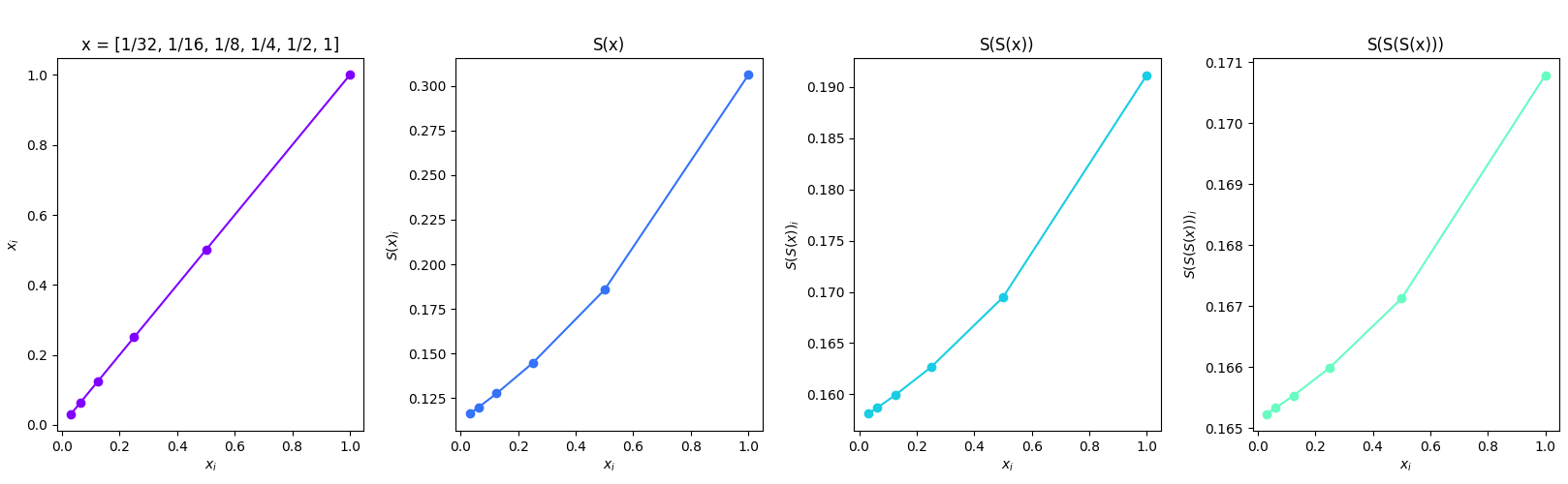
Note that while the last three diagrams have the same shape, their ranges are different. From left to right, the ranges are $[0.116, 0.306]$, $[0.158, 0.191]$, and $[0.165, 0.171]$, respectively. Each step of the transformation takes the lower and upper bounds closer to $\frac{1}{6} = 0.1666$, and the standard deviation closer to zero. The standard deviations for $S(\mathbf{x})$, $S^2(\mathbf{x})$ and $S^3(\mathbf{x})$ are $0.0665$, $0.0116$, and $0.00195,$ respectively. If we zoom out and change the plots to have the same aspect ratio, we see that the curve approaches a straight horizontal line.
The choice of the initial input vector is not important, as we see in the following diagram, which shows the result of applying softmax to $\mathbf{x} = [1, 2, 4, 8, 16, 32]$, up to 3 times:
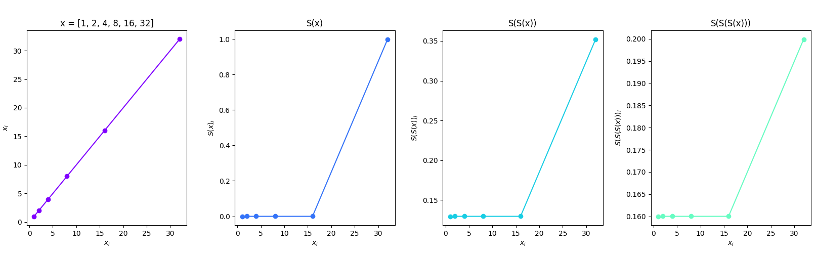
Again, the shapes have remained the same, but the ranges have shrunk.
So applying softmax on a probability distribution does not buy us anything! It only gets us closer to a uniform distribution, which means a smaller standard deviation for the output. Not that any of the neural networks I’ve seen uses softmax in this fashion, but in a deep neural network, a very small standard deviation often contributes to vanishing gradients, whereas larger standard deviations can result in more resistance against noise. Although seemingly not directly applicable anywhere in the design of a neural network, this experiment did help me better understand the behavior of softmax.
We want to find vectors $\mathbf{x}$, such that: $$ S(\mathbf{x}) = \mathbf{x} $$ Plugging in the equation of softmax, this means that for all elements $x_i$ in $\mathbf{x}$ of length $k>1$ (the $k=1$ case is obvious), we have: $$ \forall i: x_i = \frac{e^{x_i}}{\Sigma_{j=1}^{k}e^{x_j}} $$ From this, we can conclude that (1) all $x_i$’s must be in the (0, 1] range, and (2) their sum must be equal to 1. The next step is to solve the equation for each $x_i$. We can rewrite the equation as follows: $$ x_i \Sigma_{j=1}^{k}e^{x_j} = e^{x_i} $$ Or $$ x_i A_x - e^{x_i} = 0; ~where~ A_x = \Sigma_{j=1}^{k}e^{x_j} \tag{1}$$ This is still too complicated to solve, particularly because of the presence of $A_x$, which is dependent on vector $\mathbf{x}$. Let’s consider a simpler problem.
What are the roots of function $ f(z) = az-e^{z}$?
The following diagram shows the graph of $f(.)$ for a few positive values of $a$. Note that $f(.)$ represents a class of functions that vary depending on the value of $a$, and it is more accurate to include $a$ as a parameter or subscript of $f$ in the notation, but I decided to omit that to keep the notation simpler.
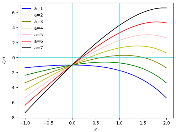
Let’s take a closer look at the $ln(a)>1$ case. We know that in this case $f(.)$ has two roots. Let’s call them $z_1$ and $z_2$, and without loss of generality, assume $z_1 < z_2$. We know that the maximum of $f(.)$ has to be between these two points. In other words, we have $z_1 < ln(a) < z_2$. We can also see this in the diagram. From this, and the fact that $ln(a)>1$, we conclude that $z_2 > 1$. The other root, $z_1$, may be greater than, less than, or equal to 1. Therefore, for any $a$, such that $ln(a)>1$, $f(.)$ has at most one root in the (0, 1] range.
Now let’s go back to equation (1) above. In this equation, $A_x= \Sigma_{j=1}^{k}e^{x_j}$. For $k \ge 3$, this means that $A_x>k>e$, and therefore, $ln(A_x)>1$. We can also show that this is true for $k=2$, and thus $\forall k>1: ln(A_x)>1$. Moreover, as stated before, all $x_i$’s are in the (0, 1] range.
Putting these together, we conclude that $x_i.A_x-e^{x_i}=0$ has at most one solution, and for $S(\mathbf{x})=\mathbf{x}$ to hold, all $x_i$’s in $\mathbf{x}$ must equal that single solution. Let's call this solution $x_A$. Then we have: $$ x_1 = x_2 = ... = x_k = x_A $$ We also know that the sum of all $x_i$’s is equal to 1, so we have $k.x_A=1$. Therefore, $x_A=\frac{1}{k}$ and: $$ \forall i: x_i = \frac{1}{k} $$ $$\tag*{$\blacksquare$}$$
The impact of softmax on mean and standard deviation
Above, we briefly touched upon how starting from a vector, and repeatedly applying softmax on its output affects the standard deviation. Now let’s see if we can work out a formula for computing the standard deviation of $S(\mathbf{x})$.
When it comes to computing standard deviation, we always start from the mean. For any input vector $\mathbf{x}$ of length $k$, the mean of $S(\mathbf{x})$ is $\frac{1}{k}$. This is because, as we saw at the beginning, the sum of elements of $S(\mathbf{x})$ is 1.
With $\mu(S(\mathbf{x}))=\frac{1}{k}$, we can compute the standard deviation of $S(\mathbf{x})$, or rather its variance, as follows:
\[\sigma^2(S(\mathbf{x})) = \frac{1}{k} \Sigma_{i=1}^k \Big(S(\mathbf{x})_i - \frac{1}{k} \Big)^2\]Expanding the quadratic term, and moving the terms around, we arrive at the following formula for the variance of $S(\mathbf{x})$:
\[\sigma^2(S(\mathbf{x})) = \frac{1}{k}\Sigma_{i=1}^k S(\mathbf{x})_i^2 - \frac{1}{k^2}\]Let $\mathbf{s}=S(\mathbf{x})$, and $\mathbf{r} = S(\mathbf{s}) = S(S(\mathbf{x}))$. Using the formula above, we have:
\[\sigma^2(\mathbf{s}) = \frac{1}{k}\Big(\Sigma_{i=1}^k s_i^2 - \frac{1}{k}\Big)\] \[\sigma^2(\mathbf{r}) = \frac{1}{k}\Big(\Sigma_{i=1}^k r_i^2 - \frac{1}{k}\Big)\]In the general case $\sigma^2(\mathbf{s}) \neq \sigma^2(\mathbf{r})$. This is in contrast to many normalization functions that, when applied to an already normalized vector, do not produce a new output, and thus, do not affect the variance and standard deviation of the data. For softmax, $\sigma(\mathbf{s})$ and $\sigma(\mathbf{r})$ will be equal, only when $\mathbf{s}$ is a uniform distribution.
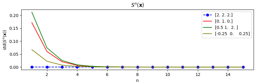
To better understand the impact of softmax on the standard deviation, the following diagram shows how the standard deviation of $S^n(\mathbf{x})$ changes as $n$ grows from 1 to 16 (recall that $S^n(.)$ is the result of applying $S(.)$ to its output, $n$ times). The diagram shows changes in standard deviation for four starting vectors of length 3, as we increase $n$. We see that, as expected, in all cases, the standard deviation converges to 0.
We can repeat the experiment for $S(c.\mathbf{x})$. Reusing the four starting vectors as in the previous experiment, the following diagram shows how the standard deviation of $S(c.\mathbf{x})$ changes as we increase $c$ from 1 to 16.
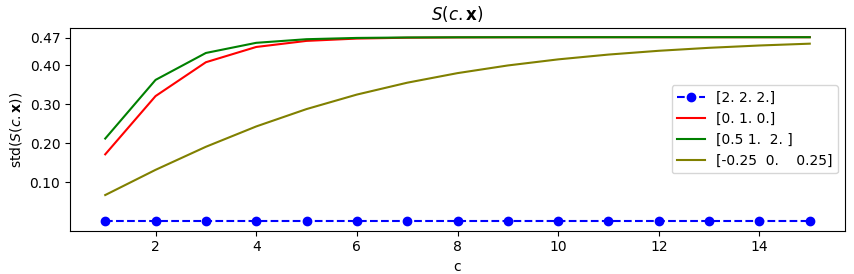
For three out of the four vectors, the standard deviation converges to $0.47$. This is because, as we saw earlier, for large values of $c$, $S(c.\mathbf{x})$ becomes argmax, and its output approaches a one-hot vector. Standard deviation of a one-hot vector of length 3 (e.g., $[0, 0, 1]$) is indeed $0.47$. The blue line is the only exception to the convergence rule. This is because in this case, the elements of the input vector are all the same, the output of softmax is [$\frac{1}{3}$, $\frac{1}{3}$, $\frac{1}{3}$], and the scaling coefficient, $c$, has no impact on this output vector (i.e., does not bring it closer to a one-hot vector). Thus in this case, the standard deviation remains the same (i.e., zero) across different $c$’s.
We could do the same for $S(\mathbf{x}+c)$, but we know that $S(\mathbf{x}+c) = S(\mathbf{x})$. So the standard deviation would not change with changes in $c$.
Gradient and partial derivatives of softmax
In the realm of machine learning, the most important property of a function is its gradient. The gradient of a multivariate function that maps $\mathbb{R}^k$ to $\mathbb{R}$ is a vector composed of the partial derivatives of the function with respect to each of its input variables. Since softmax is a vector-valued function, we can regard each element of its output vector as a multivariate function, and form a gradient vector for it. By putting all these gradients together, we get a Jacobian matrix.
Here, we are going to stick with the simpler and more familiar concept of partial derivatives, which are the building blocks of both the gradient vector and the Jacobian matrix. More specifically, we are interested in computing:
\[\frac{dS(\mathbf{x})_i}{dx_i}\]for all $1 \leq i, j \leq k$, where $k$ is the length of the input vector $\mathbf{x}$.
We have to distinguish between two cases: (1) $i = j$, and (2) $i \neq j$. Let’s start with $i=j$:
\[\frac{dS(\mathbf{x})_i}{dx_i} = \frac{d}{dx_i}\frac{e^{x_i}}{\Sigma_{j=1}^k{e^{x_j}}} = \frac{(\Sigma_{j=1}^k{e^{x_j}})e^{x_i}-e^{2x_i}}{(\Sigma_{j=1}^k{e^{x_j}})^2}\]We can simplify this to:
\[\frac{dS(\mathbf{x})_i}{dx_i} = S(\mathbf{x})_i(1-S(\mathbf{x})_i)\]Since we have $0<S(\mathbf{x})_i \le 1$, the derivative of the $i$th element of $S(\mathbf{x})$ with respect to the $i$th element of $\mathbf{x}$ is always in the range [0, 1). It becomes zero only when $\mathbf{x}$ has length 1 (i.e., it is a scalar value). Now let’s compute the derivative when $i \neq j$. We have:
\[\forall k> 1, i \neq j: \frac{dS(\mathbf{x})_i}{dx_j} = \frac{-e^{x_i}e^{x_j}}{(\Sigma_{l=1}^k{e^{x_l}})^2}\]We can write this as:
\[\frac{dS(\mathbf{x})_i}{dx_j} = - S(\mathbf{x})_i S(\mathbf{x})_j\]As expected, this partial derivative is always negative. Putting these two cases together, if we increase one of the elements in the input vector, its corresponding element in the output will increase, while all other elements of the output will decrease.
Ok! This part was dense with formulas. Let’s look at a diagram now. It is not possible to plot these partial derivatives in the general case. So we will look at a simple example, for the sake of building intuition. Let’s consider the vector $\mathbf{x} = [0, 1, …, 31]$. We are going to take $x_0$ (I am using zero-based indexing here to be consistent with the python code that generated the diagram) and modify it, by increasing its value from -100 to 100, while keeping all other values in $\mathbf{x}$ fixed. In the following, the graphs on the top show how $S(\mathbf{x})_0$ and ${S(\mathbf{x})_3}_1$ change as we increase $S(\mathbf{x})_0$. I have chosen ${S(\mathbf{x})_3}_1$ because it gives the best visual appearance.
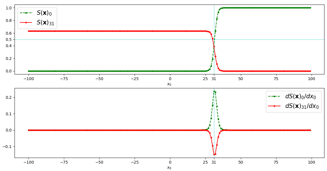
The lower graphs show how the derivatives of $S(\mathbf{x})_0$ and ${S(\mathbf{x})_3}_1$ change as we increase $x_0$.
We can take this one step further, and compute the second partial derivatives. For $i=j$, we have:
\[\frac{d^2S(\mathbf{x})_i}{d^2x_i} = S(\mathbf{x})_i(1-S(\mathbf{x})_i)(1-2S(\mathbf{x})_i)\]This formula yields a positive value, if $S(\mathbf{x})_i$ is less than $0.5$, and becomes negative only when $S(\mathbf{x})_i$ is larger than $0.5$. We can also see this in the diagram. In this example, $S(\mathbf{x})_0$ is larger than $0.5$ for $x_0>31$. At this point the derivative of $S(\mathbf{x})_0$ starts to fall, as we see in the lower diagram. Note that as $S(\mathbf{x})_0$ grows larger than $0.5$, ${S(\mathbf{x})_3}_1$ falls below $0.5$. Intuitively, this is because a probability distribution (e.g., vector $S(\mathbf{x})$) cannot have more than one value larger than $0.5$.
The second partial derivative of softmax in the $i \neq j$ case is given by the following formula:
\[\frac{d^2S(\mathbf{x})_i}{d^2x_j} = S(\mathbf{x})_i S(\mathbf{x})_j (2S(\mathbf{x})_j - 1)\]According to this formula, the second derivative of ${S(\mathbf{x})_3}_1$ with respect to $x_0$ is positive only when $S(\mathbf{x})_0>1/2$. As we saw above, this first happens after $x_0=31$ (i.e., at $x_0=32$), and that is where ${dS(\mathbf{x})_3}_1/dx_0$ starts to grow, as we see in the lower diagram. Note that despite this, the value of ${dS(\mathbf{x})_3}_1/dx_0$ remains negative, and ${S(\mathbf{x})_3}_1$ continues to decline after this point, as shown by the red line in the upper diagram.
The “S”-shaped curve in the upper diagram might have reminded you of sigmoid. Here are the formulas for sigmoid ($\sigma(x)$), and its first and second derivatives:
\[\sigma(x) = \frac{1}{1+e^{-x}}\] \[\sigma'(x) = \sigma(x)(1-\sigma(x))\] \[\sigma''(x) = \sigma(x)(1-\sigma(x))(1 - 2\sigma(x))\]Despite the seeming resemblance between sigmoid and softmax, they are very different functions. Sigmoid operates on scalars, and maps them to scalars. Even though in the machine learning world the input to sigmoid is often a vector, sigmoid is applied to each element of the vector independently. Changes to one element of the input vector has no impact on the outputs of other elements. This is in contrast to softmax where, as we see in the red curves in the diagram above, changes to one element of the vector affects the output for all other elements.
We could continue studying other properties of softmax, for instance its inverse (does it even have an inverse?). But I am going to stop this part here!
Softmax in higher dimensions
So far, we have been only considering 1-dimensional arrays. But in general, we could apply softmax to any n-dimensional (also written as n-D) array. In fact implementations of softmax in popular python packages take an n-D array as input. In tensorflow terminology, an n-D array is called a rank-n tensor.
The simplest n-D array is a 0-D array, or a scalar. Applying softmax to any scalar gives 1. If we plot $S(\mathbf{x})$ for $\mathbf{x} \in \mathbb{R}$, we’ll get the horizontal line $y=1$. Note that in practice, a 0-D array behaves the same as a 1-D array of length 1.
Now let’s move on to the 2-D space, and apply softmax to points on the unit circle! Because, why not?!
If we have $k$ points, then the input vector will be a 2-D array of the shape $(2, k)$ or $(k, 2)$, depending on how you want to arrange the points. For this example, I use $(2, k)$, to keep the code for generating the points and plotting them simpler. The domain of softmax in this case is $\mathbb{R}^{2 \times k}$. The following snippet generates such an input vector:
x = np.arange(-1, 1.01, 0.02)                # 101 points in [-1, 1].
y = np.sqrt(np.absolute(1 - np.power(x, 2))) # The upper semicircle.

x = np.concatenate((x, np.flip(x)), axis=None)
y = np.concatenate((y, np.flip(-y)), axis=None)
v = np.array([x, y])
As shown in the code, we have: $y = \pm \sqrt{1- x^2}$. The vector we want to pass into softmax is $\mathbf{v} = [\mathbf{x}, \mathbf{y}]$. In the code snippet above, vector $\mathbf{v}$ has shape $(2, 202)$.
With such an input vector, we have a few options when applying softmax. We can either treat the entire content of the array as a single vector, and apply softmax on the flattened 1-D vector, or apply softmax on each dimension independently. In scipy.special, which is the package I am using, this is done using the axis argument to the softmax function. Note that regardless of our choice of axis, softmax from scipy.special returns an array with the same shape as the input.
Let’s start with applying softmax to the entire vector:
from scipy.special import softmax

s = softmax(v, axis=None)
print(s.sum()) # Prints 1.0
print(s.shape) # Prints (2, 202)
In this code snippet, we use $\mathbf{s}$ to denote the result of applying softmax to $\mathbf{v}$. As expected, after the transformation, the sum of all the elements in $\mathbf{s}$ is 1. To see the effect of applying softmax on $\mathbf{v}$, the following diagram shows two curves. The one on the left plots $\mathbf{y}$ (i.e., $\mathbf{v}[1]$) over $\mathbf{x}$ (i.e., $\mathbf{v}[0]$). As expected, the result is a circle. On the right, we do the same for elements of $\mathbf{s}$. We plot $\mathbf{s}[1]$ on the y-axis, over $\mathbf{s}[0]$ on the x-axis.
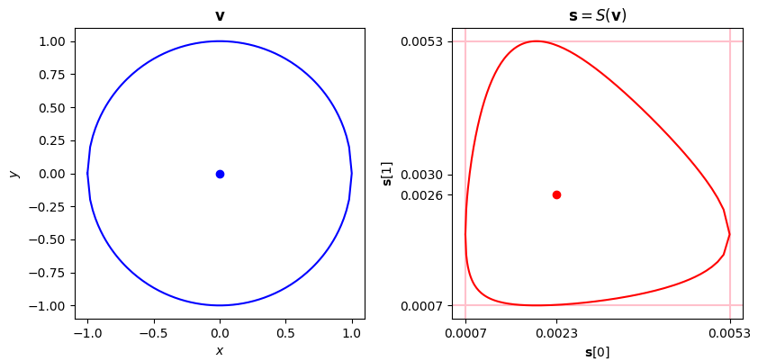
After the transformation we have an asymmetrical and skewed egg-shaped curve. In our original input, the points on the upper circle have positive values on the y-axis. These are sines of angles between 0 and $\pi$. After the transformation, these values have become smaller, but they are proportionately larger than the y-values of the lower half of the transformed shape. The points on the lower semicircle, on the left, have negative values on the y-axis. After the transformation, these values have become small positive values, all in the range $[0.0007, 0.00195]$. The x-axis also shrank from [-1, 1] to $[0.0007, 0.0053]$.
The following table reports the min, max, mean, and standard deviations of $\mathbf{x}$, $\mathbf{y}$, $\mathbf{v}$ and their softmax transformations, $\mathbf{s}$, $\mathbf{s}[0]$, $\mathbf{s}[1]$.
| Vector | Min | Max | Mean | Standard deviation |
|---|---|---|---|---|
| $\mathbf{x}$ | -1.0 | 1.0 | 0.0 | 0.5831 |
| $\mathbf{y}$ | -1.0 | 1.0 | 0.0 | 0.8124 |
| $\mathbf{v}$ | -1.0 | 1.0 | 0.0 | 0.7071 |
| $\mathbf{s} = S(\mathbf{v}) $ | 0.00072 | 0.0053 | 0.00247 | 0.0016 |
| $\mathbf{s}[0]$ (corresponding to $\mathbf{x}$) | 0.00072 | 0.0053 | 0.00230 | 0.0013 |
| $\mathbf{s}[1]$ (corresponding to $\mathbf{y}$) | 0.00072 | 0.0053 | 0.00265 | 0.0018 |
Vector $\mathbf{v}$ has $404$ elements. So the mean of its softmax transformation, $\mathbf{s}$ , is $\frac{1}{404} (=0.00247)$. But $\mathbf{s}[0]$ and $\mathbf{s}[1]$ have different means, which should not be surprising, because the input vectors $\mathbf{x}$ and $\mathbf{y}$ don’t have the exact same values, as we can see from the difference in their standard deviations. Note that the ranges for $\mathbf{s}$, $\mathbf{s}[0]$ and $\mathbf{s}[1]$ would not be so small if we had fewer points in $\mathbf{v}$. But then the diagrams would not be as smooth.
From the table, we see that $\mathbf{s}[0]$ and $\mathbf{s}[1]$ have the same min and max, and these are in fact softmax transformations of -1 and 1 for our input vector $\mathbf{v}$. In other words:
\[argmin(S(\mathbf{v})) = argmin(\mathbf{v})\] \[argmax(S(\mathbf{v})) = argmax(\mathbf{v})\]Visually, the highest and lowest points of the original circle have become the highest and lowest points in the new shape, respectively. Likewise, the leftmost and rightmost points of the original circle have become the leftmost and rightmost points in the new shape.
However, their alignment with the center has changed. In the circle, the x-coordinate of the highest and lowest points is the same as the x-coordinate of the center, which is at $(0, 0)=(\mu(\mathbf{x}), \mu(\mathbf{y}))$. In the transformed shape, the x-coordinate of the highest and lowest points is $0.00195$ (under the transformation $0$ is mapped to $0.00195$), which is different from the x-coordinate of the new center at $(0.00230, 0.00265)=(\mu(\mathbf{s}[0]), \mu(\mathbf{s}[1]))$. We see the same misalignment for the y-coordinate of the leftmost and rightmost points in the new shape.
In addition to this misalignment with respect to the center, the points on the curve no longer have the same distance to the center. The following diagram shows the distance of each point on the transformed shape to its center (indicated by the red dot in the diagram above), starting from the leftmost point (corresponding to $(-1, 0)$ in the circle) and visiting all points on the curve in a clockwise traversal.
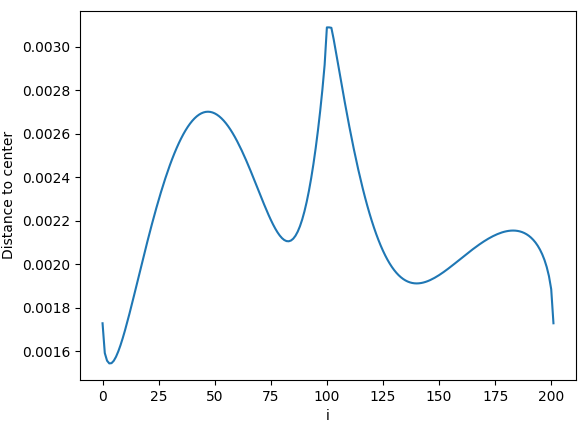
We see the first peak at the point corresponding to $(0, 1)$ in the original circle. The second peak corresponds to $(1, 0)$. These two points, although being reflections of each other with respect to the $x=y$ line, have different distances from the center. This is because the x- and y-coordinates of the center in the transformed shape are different.
We can talk more about this curve, and the curious reader is invited to analyze it further, but for now, let’s move on to applying softmax along each row of our 2-D vector $\mathbf{v}$, independently.
This is effectively the same as applying softmax to $\mathbf{x}$ and $\mathbf{y}$ vectors separately. As shown in the following snippet, we do this by setting axis=1.
s = softmax(v, axis=1)
print(s.sum()) # Prints 1.9999999999999998
print(s.shape) # Prints (2, 202)
The sum of all elements of $\mathbf{s}$ in this case is $2.0$, instead of $1.0$ that we saw in the previous case. When we plot $\mathbf{s}[1]$ over $\mathbf{s}[0]$, we see a similar shape as before, but the ranges of the transformed values are different. On the x-axis we have $[0.00154, 0.0114]$, and on the y-axis we have $[0.00135, 0.0099]$.
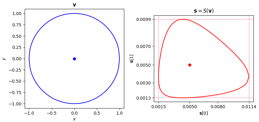
As before, let’s take a quick look at min, max, mean, and standard deviation after the transformation:
| Vector | Min | Max | Mean | Standard deviation |
|---|---|---|---|---|
| $\mathbf{s} = S(\mathbf{v}) $ | 0.00135 | 0.01141 | 0.00495 | 0.00314 |
| $\mathbf{s}[0]$ (corresponding to $\mathbf{x}$) | 0.00154 | 0.01141 | 0.00495 | 0.00280 |
| $\mathbf{s}[1]$ (corresponding to $\mathbf{y}$) | 0.00135 | 0.00995 | 0.00495 | 0.00344 |
Comparing this table with the previous one we see that the min and max values are roughly twice that of the previous case. Also, the means of all vectors in this case are equal to $\frac{1}{202}$. Can you explain why?
The last option we have for applying softmax to our vector $\mathbf{v}$, is to apply it on each point, independently.
s = softmax(v, axis=0)
print(s.sum()) # Prints 202.0
print(s.shape) # Prints (2, 202)
The sum of all elements of $\mathbf{s}$ in this case is $202.0$ (we have $202$ points in vector $\mathbf{v}$). Since the output of softmax is always a valid probability distribution, for each index $i \in [0, 201]$, we have:
\[s[0]_i + s[1]_i = 1\]In other words, coordinates of the points on the transformed shape can be specified as:
\[y = 1 -x\]The softmax transformation has turned our circle into a line!
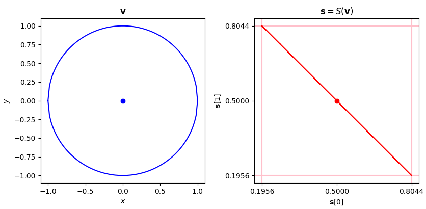
I hope you find these experiments and discussions as much fun and useful as I did. I am still trying to get my head around the egg-shaped curves. Do these shapes have a name, or any interesting properties? Let me know if you have any ideas.
Here is the jupyter notebook I used for the experiments and generating the diagrams.